6 rainfall
Last topic on decomposition models, using regression. This is monthly data, but we cannot use calendar trigonometric pairs. Months are of unequal length, and trading days don’t play a role. The length of each month is indicated in the dataset, as monthlength. The rainfall is in milimeters.
Volatility changes a bit from time to time. Higher levels of rainfall mean more volatility than lower levels. Log transformation is one option, but there are a few months that have no rainfall, and can’t take the log of 0, so change these months to 1 millimeter. Log transformation is a substantial overcorrection, where the dry months have much more variability than the wet months.
Power transformation. Alpha equal to a third, take the cubed root. Then fit a model with a trend component and determine trend is not sig. Reason the R-squared is so low is because not a lot of vertical dispersion. Fluctuations are relatively constant. the only significant components are the first two cosine sine pairs. Re-fit with just these pairs. In model 2, in the reduced model, it is 2.7150. Why didn’t this coefficient change when we dropped the pair? When the number of data sets is a multiple of 12, you have perfect lack of collinearity. The cosines are orthogonal to the sins, and any one pair is uncorrelated completely. Leads to a situation where there are no changes. The standard errors do change. Reduced model has lower R squared.
Seasonal estimates show that rainy season spans October-April.
In model 3, normal QQ plot is off. And plotting the residuals against the predicted values show megaphone shape (heteroskedasticity) so there is volatility. We need to use that square root transformation.
Does model 2 reduce to white noise? Autocorrelations of the residuals indicate reducing to white noise.
Amplitude and peak calculations ->
rain <- read.csv("/cloud/project/data/rainfall.txt")
attach(rain)
head(rain)
## year month monthlength time rainfall
## 1 1979 1 31 1 90
## 2 1979 2 28 2 193
## 3 1979 3 31 3 92
## 4 1979 4 30 4 148
## 5 1979 5 31 5 0
## 6 1979 6 30 6 88plot(ts(rainfall,start = c(1979,1), freq = 12))
modrainfall<-rainfall
 for(i in 1:length(rainfall)){
 if(rainfall[i]==0)modrainfall[i]<-rainfall[i]+1
 }
plot(ts(log(modrainfall),start=c(1979,1),freq=12))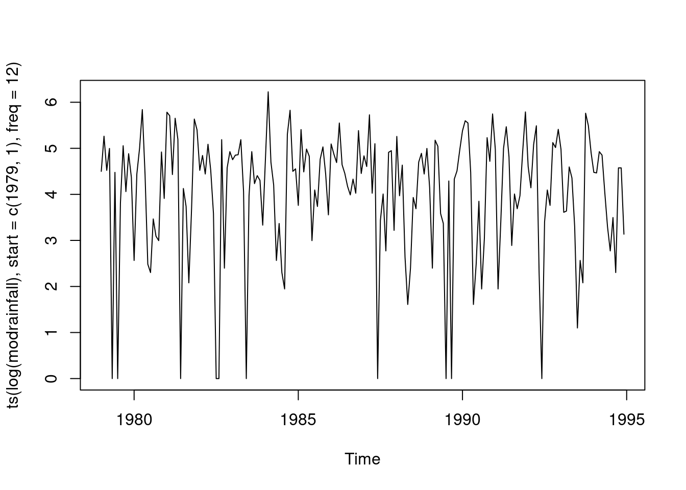
plot(ts(sqrt(modrainfall),start=c(1979,1),freq=12))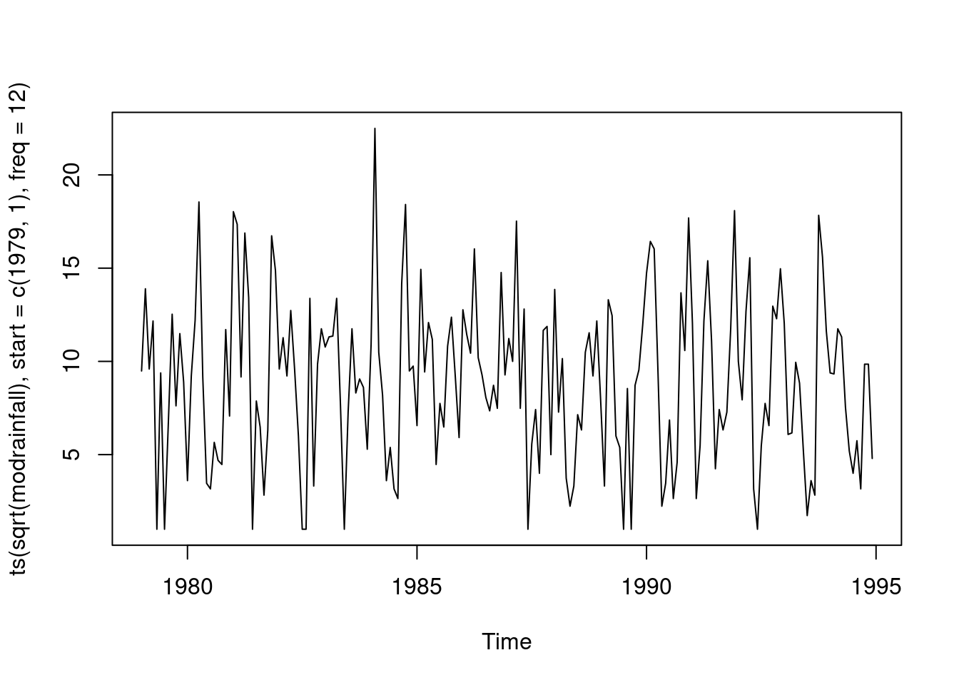
time<-as.numeric(1:length(rainfall))
cosm<-matrix(nrow=length(rainfall),ncol=6)
sinm<-matrix(nrow=length(rainfall),ncol=5)
for(i in 1:5){
 cosm[,i]<-cos(2*pi*i*time/12)
 sinm[,i]<-sin(2*pi*i*time/12)
 }
cosm[,6]<-cos(pi*time)
model1<-
lm(sqrt(rainfall)~cosm[,1]+sinm[,1]+cosm[,2]+sinm[,2]+cosm[,3]+sinm[,3
]+cosm[,4]+sinm[,4]+cosm[,5]+sinm[,5]+cosm[,6]);summary(model1)
##
## Call:
## lm(formula = sqrt(rainfall) ~ cosm[, 1] + sinm[, 1] + cosm[,
## 2] + sinm[, 2] + cosm[, 3] + sinm[, 3] + cosm[, 4] + sinm[,
## 4] + cosm[, 5] + sinm[, 5] + cosm[, 6])
##
## Residuals:
## Min 1Q Median 3Q Max
## -8.2879 -2.4459 0.0804 2.0217 11.5607
##
## Coefficients:
## Estimate Std. Error t value Pr(>|t|)
## (Intercept) 8.8849 0.2732 32.518 < 2e-16 ***
## cosm[, 1] 2.7150 0.3864 7.026 4.22e-11 ***
## sinm[, 1] 1.8291 0.3864 4.734 4.45e-06 ***
## cosm[, 2] -0.8887 0.3864 -2.300 0.022600 *
## sinm[, 2] -1.2941 0.3864 -3.349 0.000988 ***
## cosm[, 3] 0.5053 0.3864 1.308 0.192623
## sinm[, 3] -0.2137 0.3864 -0.553 0.580835
## cosm[, 4] -0.6180 0.3864 -1.599 0.111514
## sinm[, 4] 0.2062 0.3864 0.534 0.594282
## cosm[, 5] -0.1749 0.3864 -0.453 0.651444
## sinm[, 5] -0.1179 0.3864 -0.305 0.760609
## cosm[, 6] 0.1439 0.2732 0.526 0.599196
## ---
## Signif. codes: 0 '***' 0.001 '**' 0.01 '*' 0.05 '.' 0.1 ' ' 1
##
## Residual standard error: 3.786 on 180 degrees of freedom
## Multiple R-squared: 0.3424, Adjusted R-squared: 0.3022
## F-statistic: 8.52 on 11 and 180 DF, p-value: 5.002e-12model2<-
lm(sqrt(rainfall)~cosm[,1]+sinm[,1]+cosm[,2]+sinm[,2]);summary(model2)##
## Call:
## lm(formula = sqrt(rainfall) ~ cosm[, 1] + sinm[, 1] + cosm[,
## 2] + sinm[, 2])
##
## Residuals:
## Min 1Q Median 3Q Max
## -8.504 -2.386 0.132 2.157 11.344
##
## Coefficients:
## Estimate Std. Error t value Pr(>|t|)
## (Intercept) 8.8849 0.2721 32.655 < 2e-16 ***
## cosm[, 1] 2.7150 0.3848 7.056 3.24e-11 ***
## sinm[, 1] 1.8291 0.3848 4.753 3.98e-06 ***
## cosm[, 2] -0.8887 0.3848 -2.310 0.022001 *
## sinm[, 2] -1.2941 0.3848 -3.363 0.000935 ***
## ---
## Signif. codes: 0 '***' 0.001 '**' 0.01 '*' 0.05 '.' 0.1 ' ' 1
##
## Residual standard error: 3.77 on 187 degrees of freedom
## Multiple R-squared: 0.3225, Adjusted R-squared: 0.308
## F-statistic: 22.26 on 4 and 187 DF, p-value: 4.806e-15anova(model2,model1)## Analysis of Variance Table
##
## Model 1: sqrt(rainfall) ~ cosm[, 1] + sinm[, 1] + cosm[, 2] + sinm[, 2]
## Model 2: sqrt(rainfall) ~ cosm[, 1] + sinm[, 1] + cosm[, 2] + sinm[, 2] +
## cosm[, 3] + sinm[, 3] + cosm[, 4] + sinm[, 4] + cosm[, 5] +
## sinm[, 5] + cosm[, 6]
## Res.Df RSS Df Sum of Sq F Pr(>F)
## 1 187 2658.0
## 2 180 2580.1 7 77.885 0.7762 0.608seas2<-(predict(model2)-coef(model2)[1])[1:12]
plot(ts(seas2),xlab="month",ylab="seasonal estimate")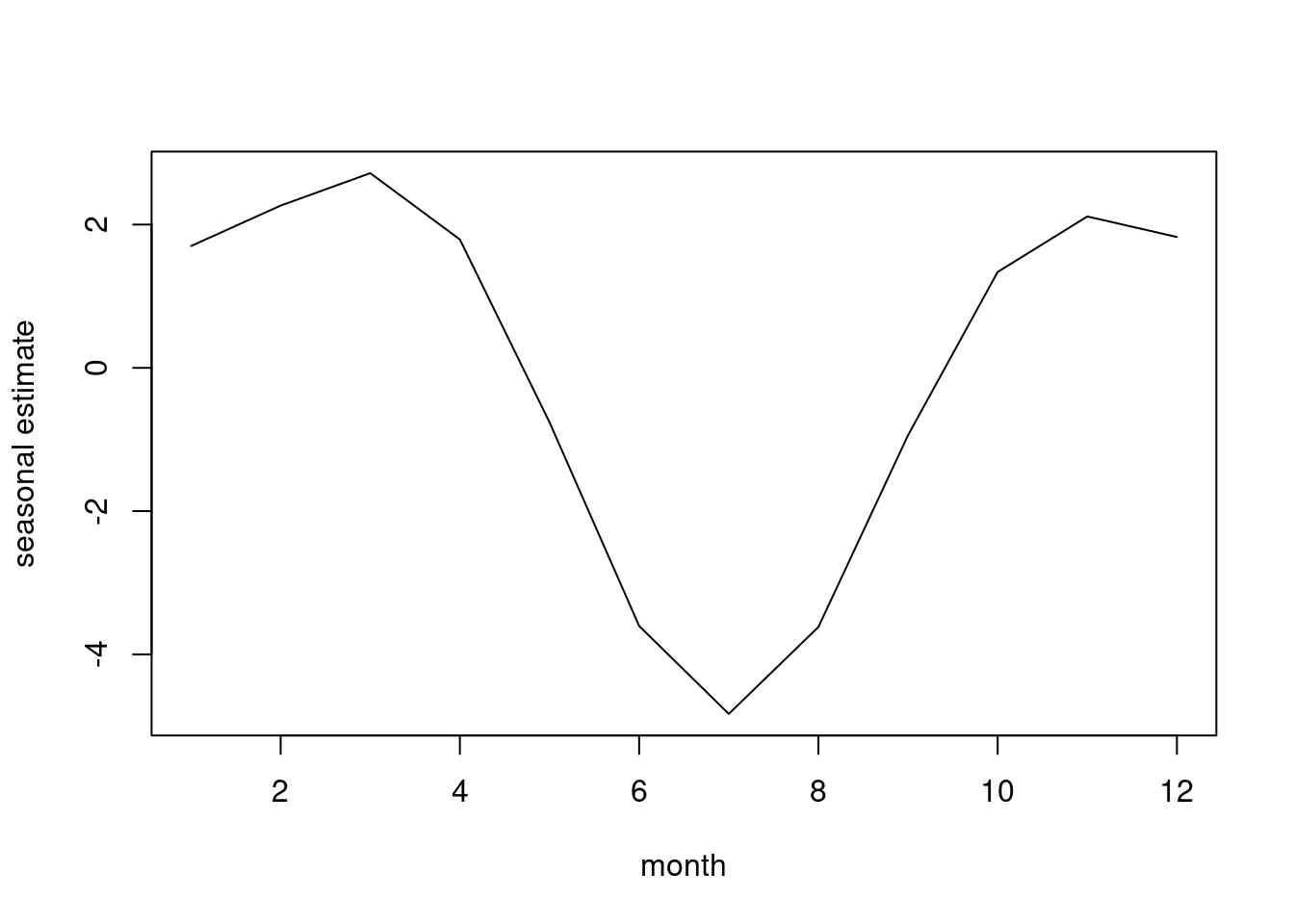
cbind(1:12,seas2)## seas2
## 1 1 1.7007794
## 2 2 2.2651957
## 3 3 2.7177618
## 4 4 1.7915266
## 5 5 -0.7604333
## 6 6 -3.6037428
## 7 7 -4.8308531
## 8 8 -3.6178537
## 9 9 -0.9403461
## 10 10 1.3385472
## 11 11 2.1130913
## 12 12 1.8263272qqnorm(resid(model2))
qqline(resid(model2))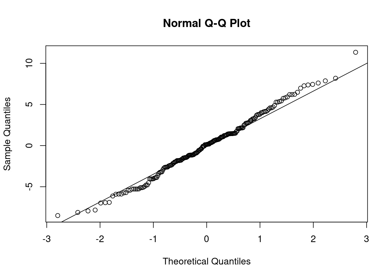
shapiro.test(resid(model2))##
## Shapiro-Wilk normality test
##
## data: resid(model2)
## W = 0.99356, p-value = 0.5691model3<-
lm(rainfall~cosm[,1]+sinm[,1]+cosm[,2]+sinm[,2]);summary(model3)##
## Call:
## lm(formula = rainfall ~ cosm[, 1] + sinm[, 1] + cosm[, 2] + sinm[,
## 2])
##
## Residuals:
## Min 1Q Median 3Q Max
## -132.28 -43.80 -10.95 30.08 366.72
##
## Coefficients:
## Estimate Std. Error t value Pr(>|t|)
## (Intercept) 99.375 5.487 18.112 < 2e-16 ***
## cosm[, 1] 44.334 7.759 5.714 4.30e-08 ***
## sinm[, 1] 33.646 7.759 4.336 2.37e-05 ***
## cosm[, 2] -13.964 7.759 -1.800 0.07353 .
## sinm[, 2] -21.227 7.759 -2.736 0.00682 **
## ---
## Signif. codes: 0 '***' 0.001 '**' 0.01 '*' 0.05 '.' 0.1 ' ' 1
##
## Residual standard error: 76.02 on 187 degrees of freedom
## Multiple R-squared: 0.2495, Adjusted R-squared: 0.2335
## F-statistic: 15.54 on 4 and 187 DF, p-value: 5.379e-11qqnorm(resid(model3))
qqline(resid(model3))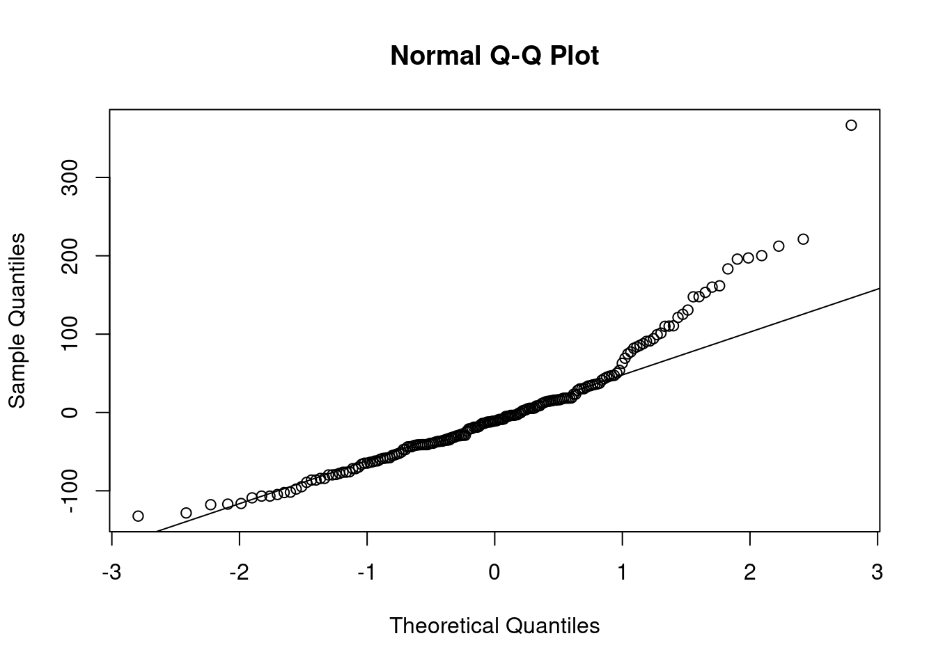
plot(predict(model3),resid(model3),xlab="predicted
rainfall",ylab="rainfall residual",main="Residual by Predicted Plot")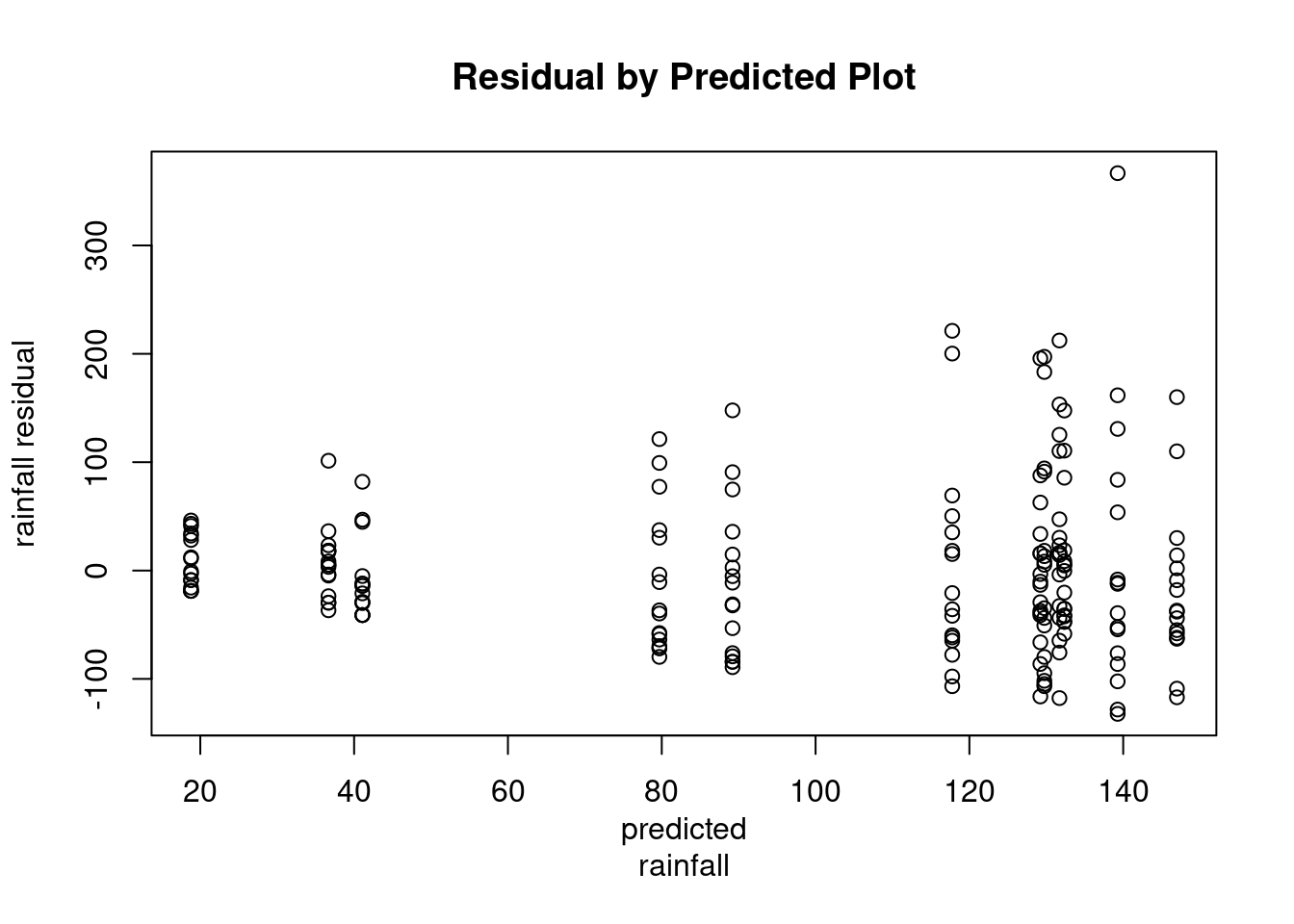
plot(ts(resid(model2),start=c(1979,1),freq=12))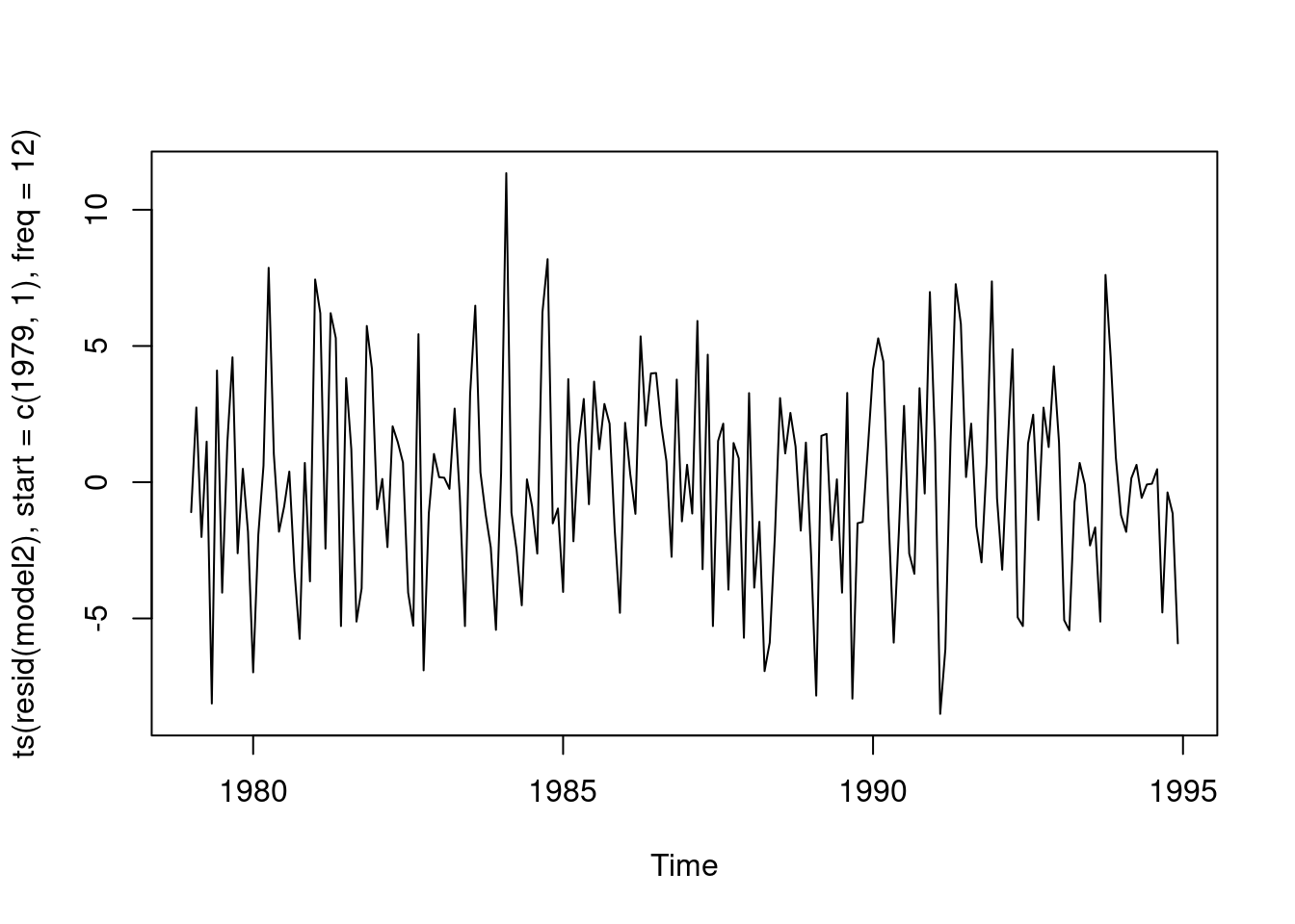
acf(resid(model2))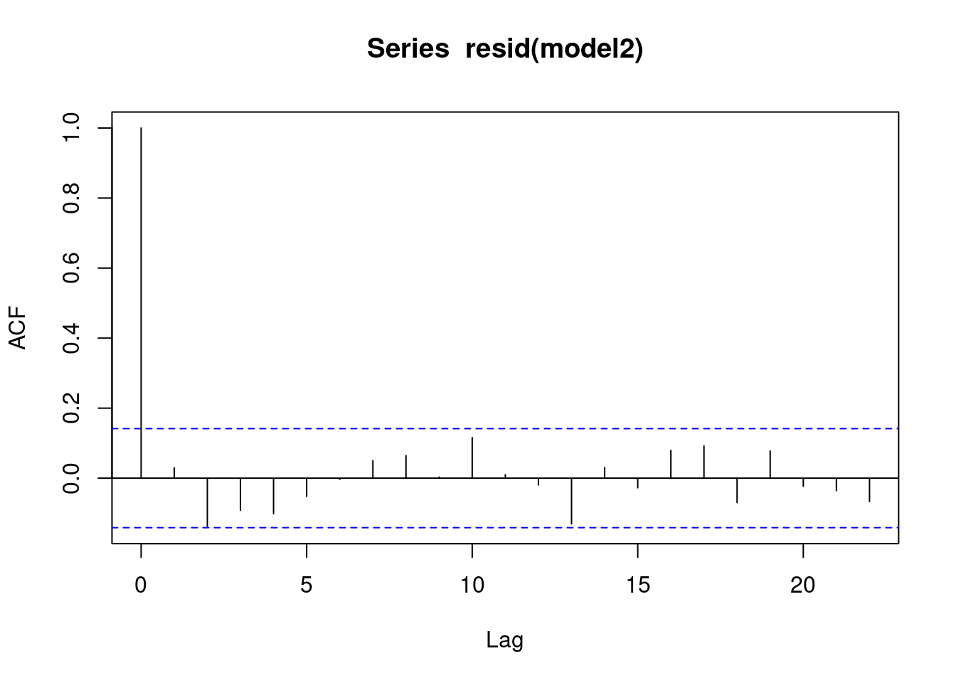
Calendar adjustment: will just deal with the length of the months.
adjrainfall<-rainfall*365.25/(12*monthlength)
model4<-
lm(sqrt(adjrainfall)~cosm[,1]+sinm[,1]+cosm[,2]+sinm[,2]);summary(model4)
##
## Call:
## lm(formula = sqrt(adjrainfall) ~ cosm[, 1] + sinm[, 1] + cosm[,
## 2] + sinm[, 2])
##
## Residuals:
## Min 1Q Median 3Q Max
## -8.5007 -2.3860 0.1723 2.0834 11.7860
##
## Coefficients:
## Estimate Std. Error t value Pr(>|t|)
## (Intercept) 8.8943 0.2730 32.581 < 2e-16 ***
## cosm[, 1] 2.7314 0.3861 7.075 2.91e-11 ***
## sinm[, 1] 1.8798 0.3861 4.869 2.38e-06 ***
## cosm[, 2] -0.9312 0.3861 -2.412 0.01683 *
## sinm[, 2] -1.2636 0.3861 -3.273 0.00127 **
## ---
## Signif. codes: 0 '***' 0.001 '**' 0.01 '*' 0.05 '.' 0.1 ' ' 1
##
## Residual standard error: 3.783 on 187 degrees of freedom
## Multiple R-squared: 0.3256, Adjusted R-squared: 0.3112
## F-statistic: 22.57 on 4 and 187 DF, p-value: 3.162e-15seas22<-2*seas2*coef(model2)[1]+seas2*seas2
seas22<-seas22-mean(seas22)
seas22## 1 2 3 4 5 6 7 8
## 26.52443 38.79242 49.08952 28.45390 -19.52505 -57.64120 -69.09644 -57.79004
## 9 10 11 12
## -22.41606 18.98672 35.42361 29.19820seas4<-(predict(model4)-coef(model4)[1])[1:12]
seas42<-2*seas4*coef(model4)[1]+seas4*seas4
seas42<-seas42-mean(seas42)
seas42## 1 2 3 4 5 6 7 8
## 27.36490 40.93254 51.17789 29.00696 -20.26817 -58.46723 -69.60506 -58.04449
## 9 10 11 12
## -22.70282 18.03920 34.03326 28.53301Model 1: model without the square root transformation:
\[ y_t = \alpha + S_t + \epsilon_t \]
Model 2: alpha hat + sub_t
\[ y_t = \alpha + \hat{S}_t \]
Model 3: model with the square root transformation
\[ \sqrt(y_t) = \alpha^* + S_t^* + \epsilon_t^* \]
model 4:
\[ pred(\sqrt(y_t) = \hat{\alpha}^* + \hat{S}^* \]
Model 5
\[ \hat\alpha +\hat{S}_t = (\alpha + \hat{S}_t)^2 = \alpha^2 \]
seas22<-2*seas2*coef(model2)[1]+seas2*seas2
seas22<-seas22-mean(seas22)
seas22
## 1 2 3 4 5 6 7 8
## 26.52443 38.79242 49.08952 28.45390 -19.52505 -57.64120 -69.09644 -57.79004
## 9 10 11 12
## -22.41606 18.98672 35.42361 29.19820seas4<-(predict(model4)-coef(model4)[1])[1:12]
seas42<-2*seas4*coef(model4)[1]+seas4*seas4
seas42<-seas42-mean(seas42)
seas42## 1 2 3 4 5 6 7 8
## 27.36490 40.93254 51.17789 29.00696 -20.26817 -58.46723 -69.60506 -58.04449
## 9 10 11 12
## -22.70282 18.03920 34.03326 28.53301boxplot(adjrainfall~month)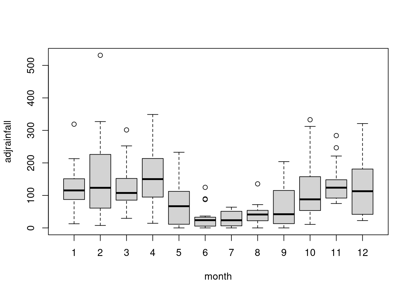
means<-tapply(adjrainfall,month,mean)
stddevs<-tapply(adjrainfall,month,sd)
cbind(1:12,means,stddevs)
## means stddevs
## 1 1 125.00239 72.88222
## 2 2 156.10230 137.80490
## 3 3 126.29108 70.94935
## 4 4 159.67005 89.63917
## 5 5 76.58468 69.14656
## 6 6 31.70573 36.94440
## 7 7 27.98286 23.97281
## 8 8 42.71069 32.26306
## 9 9 68.29414 67.18730
## 10 10 118.25214 94.88598
## 11 11 137.66628 61.98290
## 12 12 127.02747 96.22035wts<-rep(1/stddevs,times=16)
modelw1<-lm(adjrainfall~cosm[,1]+sinm[,1]+cosm[,2]+sinm[,2]+cosm[,3]+sinm[,3]+cosm[,4]+sinm[,4]+cosm[,5]+sinm[,5]+cosm[,6],weights=wts)
summary(modelw1
)##
## Call:
## lm(formula = adjrainfall ~ cosm[, 1] + sinm[, 1] + cosm[, 2] +
## sinm[, 2] + cosm[, 3] + sinm[, 3] + cosm[, 4] + sinm[, 4] +
## cosm[, 5] + sinm[, 5] + cosm[, 6], weights = wts)
##
## Weighted Residuals:
## Min 1Q Median 3Q Max
## -15.364 -5.702 -1.373 3.389 31.943
##
## Coefficients:
## Estimate Std. Error t value Pr(>|t|)
## (Intercept) 99.7742 5.1353 19.429 < 2e-16 ***
## cosm[, 1] 44.7047 6.9660 6.418 1.19e-09 ***
## sinm[, 1] 35.0058 7.5472 4.638 6.74e-06 ***
## cosm[, 2] -15.1003 7.1769 -2.104 0.03677 *
## sinm[, 2] -20.2614 7.3469 -2.758 0.00642 **
## cosm[, 3] 3.8913 7.7624 0.501 0.61677
## sinm[, 3] -3.6765 6.7253 -0.547 0.58528
## cosm[, 4] -11.4445 7.1769 -1.595 0.11255
## sinm[, 4] 2.5755 7.3469 0.351 0.72633
## cosm[, 5] -0.9352 6.9660 -0.134 0.89336
## sinm[, 5] -9.6838 7.5472 -1.283 0.20110
## cosm[, 6] 6.1372 5.1353 1.195 0.23362
## ---
## Signif. codes: 0 '***' 0.001 '**' 0.01 '*' 0.05 '.' 0.1 ' ' 1
##
## Residual standard error: 8.435 on 180 degrees of freedom
## Multiple R-squared: 0.3767, Adjusted R-squared: 0.3386
## F-statistic: 9.887 on 11 and 180 DF, p-value: 6.135e-14modelw2<-
lm(adjrainfall~cosm[,1]+sinm[,1]+cosm[,2]+sinm[,2],weights=wts);summary## function (object, ...)
## UseMethod("summary")
## <bytecode: 0x55cd892811a0>
## <environment: namespace:base>(modelw2)##
## Call:
## lm(formula = adjrainfall ~ cosm[, 1] + sinm[, 1] + cosm[, 2] +
## sinm[, 2], weights = wts)
##
## Coefficients:
## (Intercept) cosm[, 1] sinm[, 1] cosm[, 2] sinm[, 2]
## 99.10 44.33 31.62 -14.13 -18.40plot(ts(resid(modelw2),start=c(1979,1),freq=12))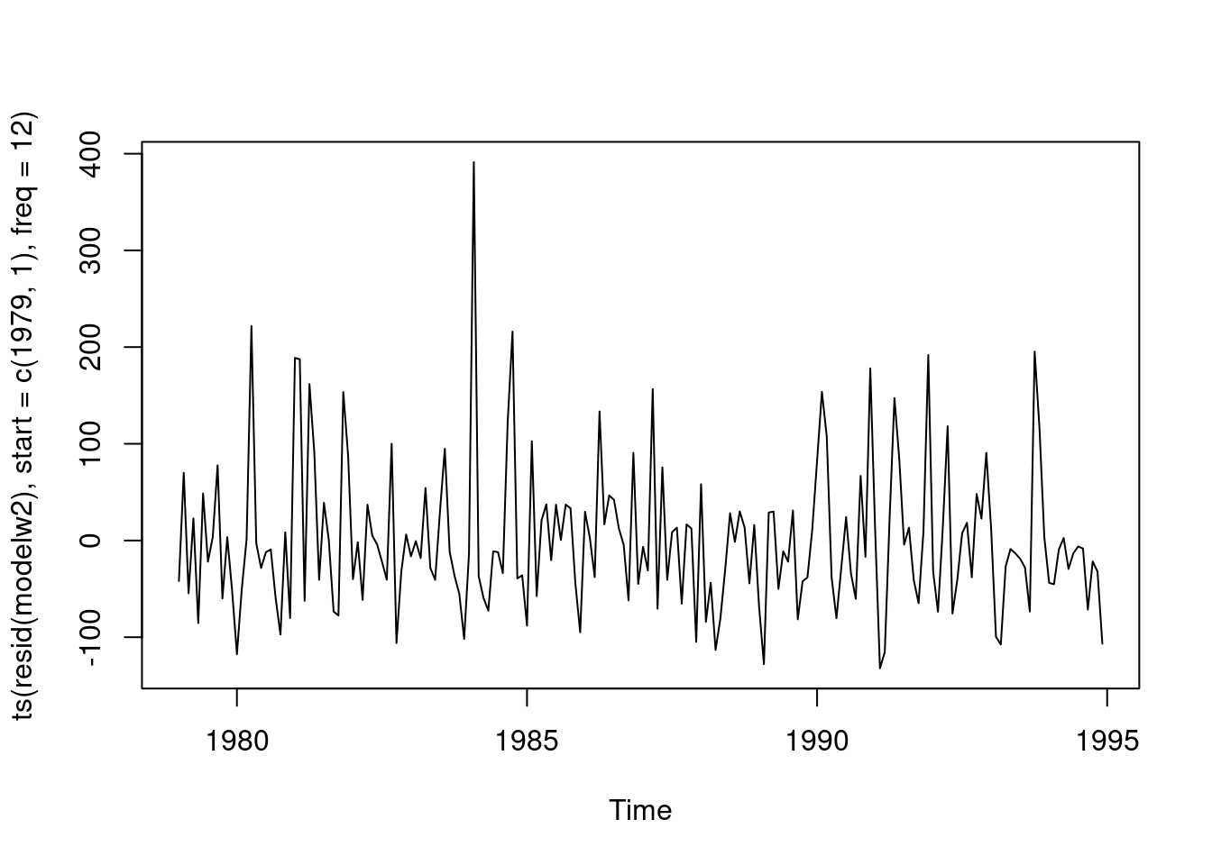
acf(ts(resid(modelw2)))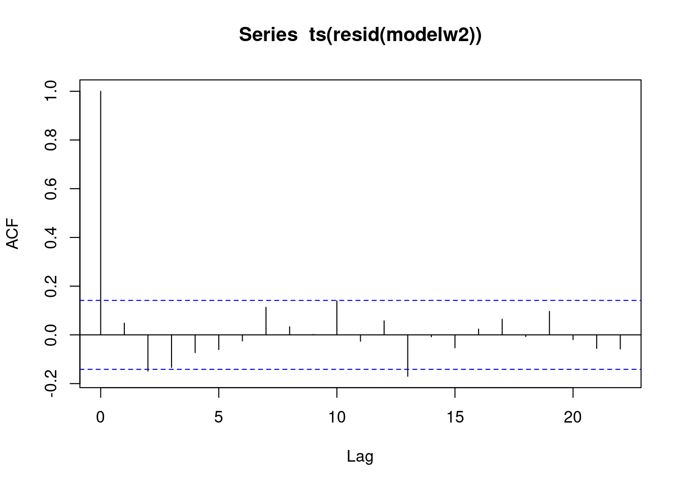
 seasw2<-(predict(modelw2)-coef(modelw2)[1])[1:12]
 seasw2
## 1 2 3 4 5 6 7 8
## 31.19822 40.67765 45.75326 28.22648 -13.70213 -58.45500 -77.20206 -58.42431
## 9 10 11 12
## -17.49609 17.77735 31.44880 30.19783 plot(ts(seas22),lty=1,lwd=2,xlab="month",ylab="seasonal",main="seasonal
estimations",col="red")
lines(ts(seas42),lty=2,lwd=2,col="blue")
lines(ts(seasw2),lty=3,lwd=2,col="green")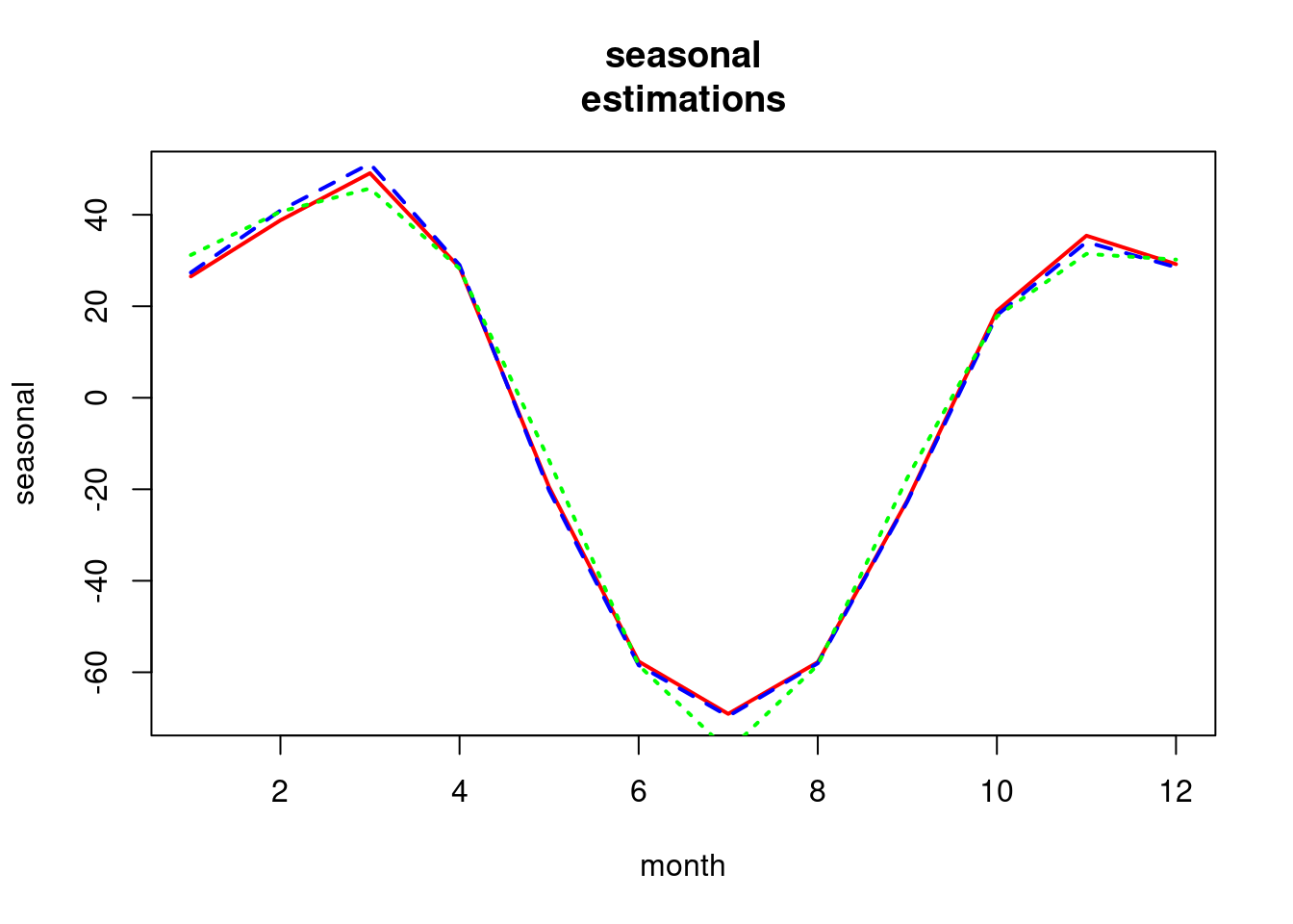
We haven’t reduced the trend in the model.
In the table: Seasonal index estimates for the sqrt, for the adj sqrt, and for the weighted least squares.