NonParametric Stats
2022-05-05
1 Hypothesis Testing
\[\begin{equation} X \sim N(\mu,\sigma^2), f(x) = \frac{1}{\sqrt{2\pi\sigma}}e-\frac{(x-\mu)^2}{2\sigma^2}, F(x) = \int_{-\infty}^{x} \frac{1}{\sqrt{2\pi\sigma}}e\frac{-(t-\mu)^2}{2\sigma^2}dt \end{equation}\]
Normal Distributions
a =0
b=1
lx=100
x=seq(-4,4,length=lx)
fx = dnorm(x,a,b)

bx = 1
dbx=dnorm(bx,a,b)
dbx
## [1] 0.2419707plot(x,fx, type = "l", xlab = "x", ylab = "f(x)", main = "Normal density functions",
las= 1)
dist_2 <- dnorm(x, mean=0, sd=4)
dist_3 <- dnorm(x, mean=1, sd=1)
dist_4 <- dnorm(x, mean=1, sd =4)
lines(x, dist_2, type = "l", col = "red")
lines(x, dist_3, type = "l", col = "green")
lines(x, dist_4, type = "l", col = "blue")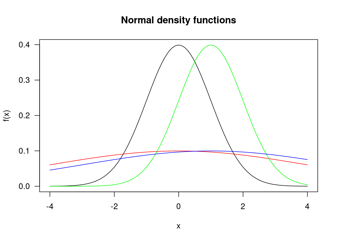
\[\begin{equation} F(x) = P(X\le x) = 1 - P(X>x) \end{equation}\]
when lower.tail == TRUE, probabiltiies are p[X<x]
## density under the curve
dnorm(x=0, mean=0, sd=1)
dnorm(0,0,2)
dnorm(0,1,1)
dnorm(0,1,2)
## probability
pnorm(0,0,1)
pnorm(0,0,2)
pnorm(0,1,1)
pnorm(0,1,2)
a=0
b=1
lx=100
x=seq(-4,4,length=lx)
fx=dnorm(x,a,b)

bx=1
dbx=dnorm(bx,a,b)

plot(x,fx,type="l",lwd=2,xlab="x",ylab="Density",main="N(0,1)",las=1,xaxt="n")
segments(bx,0,bx,dbx,lty=3)
sx=seq(-4,bx,length=lx)
polygon(c(sx,rev(sx)),c(dnorm(sx,a,b),rep(0,lx)),density=2,border=NA,lty=3)

text(-0.5,0.1,expression(P(X<=z[1-alpha])==1-alpha))
abline(h=0,lty=3)
axis(1,at=bx,label=expression(z[1-alpha]))

sx=seq(bx,4,length=lx)
polygon(c(sx,rev(sx)),c(dnorm(sx,a,b),rep(0,lx)),density=3,border=NA,
angle=-45,lty=3)
text(2.5,0.1,expression(P(X>z[1-alpha])==alpha))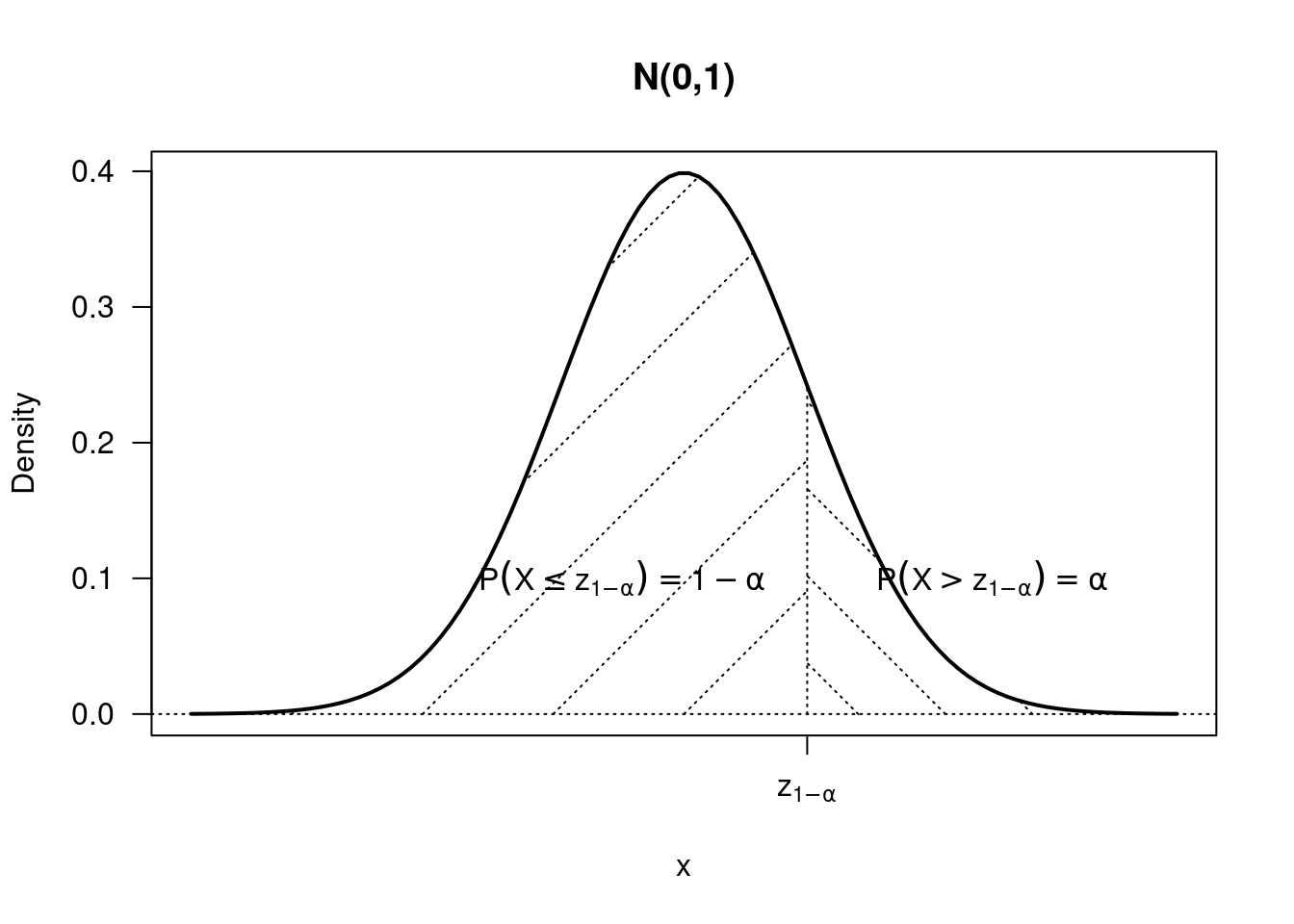
Power
Probability of rejecting \(H_0\) when it is true is type I error (falsely reject), aka significance of the test aka \(\alpha\). Probability of not reject H_0 when it is false is a type II error, \(\beta\). Power of test is \(1-\beta\).
Confidence Intervals
Confidence set with a confidence coefficient of \(1-\alpha\) is the set.
Parametric Methods
Parametric distributions with populations
\[\begin{equation} N(\mu, \sigma^2),binomial(n,p) \end{equation}\]
n=30
x=rnorm(n,mean=0,sd=1)
sort(x)
## [1] -2.21364671 -1.42634717 -1.18941984 -1.17103762 -1.12420752 -0.97980777
## [7] -0.94948592 -0.71308868 -0.46913499 -0.29407474 -0.23805540 -0.13223179
## [13] -0.10062293 -0.04215379 0.01438010 0.07546985 0.12779647 0.20875060
## [19] 0.40840068 0.43056635 0.62648993 0.66059408 0.69182638 0.70656749
## [25] 1.14932835 1.18642575 1.39787370 1.47237640 1.59213710 2.05117153xbar=mean(x)
sdx=sd(x)One sided H_0
\[\begin{equation} H_0 : \mu = \mu_0 vs. H_1: \mu > Mu_0\\ T = \frac{\sqrt(x-\mu_0)}{\sigma} \sim \text{t distribution with n-1 degrees of freedom} \\ \text{Reject null if t} > t_{n-1,1-\alpha} \\ \text{Type I error}: \alpha = P_{\mu_o}(T>t_{n-1,1-\alpha}) \\ \text{Acceptance region} : T \le t_{n-1,1-\alpha}\\ 1- \alpha = P_{\mu_0}(\frac{\sqrt{n}(\bar{X}-\mu_0)}{\hat\sigma}) \le t_{n-1,1-\alpha}\\ = P_{\mu_0}(\bar{X} - t_{n-1,1-\alpha}\frac{\hat\sigma}{\sqrt{n}} \le \mu_0) \end{equation}\]
Smaller p-value, stronger evidence against H0. Critical value for alpha of 0.05 is +-1.69. The probability that mu0=1, the upper tail probability (lower.tail = F) is 0.9999, so results have a greater chance of being due to random chance than to the data itself. Alternative: that Mo0 > Mu. If p was <.05, then the probability we would see these results are minimal (given that it is true), so we’d accept alternative. Here, not enough chance that we’d see the alternative, so fail to reject null.
alpha = 0.05
tq = qt(1-alpha, n-1)
c(qt(1-alpha, n-1), qt(alpha,n-1, lower.tail = F))
## [1] 1.699127 1.699127mu0=1
tstat=sqrt(n)*(xbar-mu0)/sdx;c(tstat,tq,pt(tstat,n-1,lower.tail=F))## [1] -5.1158989 1.6991270 0.9999908xbar-tq*sdx/sqrt(n)## [1] -0.2541157t.test(x,alternative="greater",mu=mu0)##
## One Sample t-test
##
## data: x
## t = -5.1159, df = 29, p-value = 1
## alternative hypothesis: true mean is greater than 1
## 95 percent confidence interval:
## -0.2541157 Inf
## sample estimates:
## mean of x
## 0.05856133Smaller p-value, stronger evidence against H0. The probability that mu0=-1, the upper tail probability (lower.tail = F) is <.05, so we have a lot of evidence against H0 (that these results are in the data, not due to random chance). Alternative: that Mu>-1. If <.05, then the probability we would see that is minimal (given that it is true), so we accept alternative, because seeing the alternative is not by chance. Here, very small probability of a result more extreme than the one actually observed if H0 is true. Since such a small probaility, given that we saw it in the data, then accept alternate.
mu0=-1; tstat=sqrt(n)*(xbar-mu0)/sdx
c(tstat,tq,pt(tstat,n-1, lower.tail=F))
## [1] 5.752359e+00 1.699127e+00 1.574230e-06xbar-tq*sdx/sqrt(n)## [1] -0.2541157t.test(x,alternative="greater",mu=mu0)##
## One Sample t-test
##
## data: x
## t = 5.7524, df = 29, p-value = 1.574e-06
## alternative hypothesis: true mean is greater than -1
## 95 percent confidence interval:
## -0.2541157 Inf
## sample estimates:
## mean of x
## 0.05856133Power
\[\begin{equation} \text{Reject null if }\bar{X} > \mu_0 + t_{n-1,1-\alpha}\frac{\hat\sigma}{\sqrt{n}}\\ \text{Type II error: do not reject null when it is false} \\ \beta = P_{H_1}\text{do not reject null}\\ \text{Power: the probability of rejecting null when alt is true}\\ 1-\beta = P_{\mu}(\bar{X} > \mu_0 + t_{n-1,1-\alpha}\frac{\hat\sigma}{\sqrt{n}}) \\ = P_{\mu}(\frac{\sqrt{n}(X-\mu)}{\hat\sigma} > \frac{\sqrt{n}(\mu_0 -\mu)}{\hat\sigma} + t_{n-1,1-\alpha} \end{equation}\]
alpha = 0.05
tq = qt(1-alpha, n-1)
mu0=1
mu=1.5
tv = sqrt(n)*(mu0-mu)/sdx+tq
pt(tv,n-1,lower.tail=F)
## [1] 0.8414373power.t.test(n,delta = abs(mu0-mu), sd=sdx,
type = c("one.sample"), alternative = "one.sided")##
## One-sample t test power calculation
##
## n = 30
## delta = 0.5
## sd = 1.007931
## sig.level = 0.05
## power = 0.8432604
## alternative = one.sided\[\begin{equation} t_{n-1,\beta} = \frac{\sqrt{n}(\mu_0 - \mu)}{\hat\sigma} + t_{n-1,1-\alpha}\\ n = [\frac{\hat\sigma(t_{n-1,\beta}-t_{n-1,1-\alpha})}{\mu_0-\mu}]^2 \end{equation}\]
beta =0.1
tb = qt(beta, n-1)
(sdx*(tb-tq)/(mu0-mu))^2
## [1] 36.83123power.t.test(power= 0.9, delta = abs(mu0-mu), sd = sdx,
type = c("one.sample"), alternative = "one.sided")##
## One-sample t test power calculation
##
## n = 36.19749
## delta = 0.5
## sd = 1.007931
## sig.level = 0.05
## power = 0.9
## alternative = one.sidedTwo sided H1
\[\begin{equation} H_0 : \mu = \mu_0 vs. H_1: \mu > Mu_0\\ \text{Reject null if |T|} > t_{n-1,1-\frac{\alpha}{2}} \\ \text{Acceptance region} : \frac{\sqrt{n}\mid{\bar{X} - \mu_0}\mid}{\hat\sigma} \le t_{n-1,1-\frac{\alpha}{2}}\\ 1- \alpha = P_{\mu_0}(\frac{\sqrt{n}(\bar{X}-\mu_0)}{\hat\sigma}) \le t_{n-1,1-\frac{\alpha}{2}}\\ = P_{\mu_0}(\bar{X} - t_{n-1,1-\frac{\alpha}{2}}\frac{\hat\sigma}{\sqrt{n}} \le \mu_0 \le \bar{X} + t_{n-1,1-\frac{\alpha}{2}}\frac{\hat\sigma}{\sqrt{n}}) \\ \text{Length of CI} : 2t_{n-1,1-\frac{\alpha}{2}}\frac{\hat\sigma}{\sqrt{n}} \end{equation}\]
alpha = 0.05
tq = qt(1-alpha/2, n-1)
mu0=0
tstat = sqrt(n)*(xbar-mu0)/sdx
c(tstat, tq,2*pt(abs(tstat),n-1, lower.tail =F))
## [1] 0.3182298 2.0452296 0.7525911xbar+c(-1,1)*tq*sdx/sqrt(n)## [1] -0.3178062 0.4349289t.test(x,mu=mu0)##
## One Sample t-test
##
## data: x
## t = 0.31823, df = 29, p-value = 0.7526
## alternative hypothesis: true mean is not equal to 0
## 95 percent confidence interval:
## -0.3178062 0.4349289
## sample estimates:
## mean of x
## 0.05856133mu0=1
tstat=sqrt(n)*(xbar-mu0)/sdx
c(tstat,tq,2*pt(abs(tstat),n-1,lower.tail = F))## [1] -5.115899e+00 2.045230e+00 1.837963e-05xbar + c(-1,1)*tq*sdx/sqrt(n)## [1] -0.3178062 0.4349289t.test(x,mu=mu0)##
## One Sample t-test
##
## data: x
## t = -5.1159, df = 29, p-value = 1.838e-05
## alternative hypothesis: true mean is not equal to 1
## 95 percent confidence interval:
## -0.3178062 0.4349289
## sample estimates:
## mean of x
## 0.05856133Power
alpha = 0.05; tq = qt(1-alpha/2,n-1);mu0=1;
mu=1.5;
tv0=sqrt(n)*(mu0-mu)/sdx;
pt(tv0+tq,n-1,lower.tail=F) + pt(tv0-tq,n-1);
## [1] 0.7465214power.t.test(n,delta=abs(mu0-mu), sd=sdx,
type = c("one.sample"),alternative="two.sided")##
## One-sample t test power calculation
##
## n = 30
## delta = 0.5
## sd = 1.007931
## sig.level = 0.05
## power = 0.7473605
## alternative = two.sidedpower.t.test(n,delta=abs(mu0-mu),sd=sdx,
type =c("one.sample"),alternative="two.sided",strict=T)##
## One-sample t test power calculation
##
## n = 30
## delta = 0.5
## sd = 1.007931
## sig.level = 0.05
## power = 0.7473627
## alternative = two.sided