Step up
- Data: \((x_{i}, y_{i}), i = 1.,,,,n\)
- \(y_i = m(x_{i}) + \epsilon_{i}, i =1,...,n\)
- m unknown, usually continuous and smooth
- For example, \(m(x_{i}) = \beta_{0} + \beta_{1}x_{i} +\beta_{2}x_{i}^2\)
- \(\epsilon_i\) iid from a continuous distribution, \(E\epsilon_i = 0\)
- \(E(y_{i} \mid x_{1}) = m(x_{i})\)
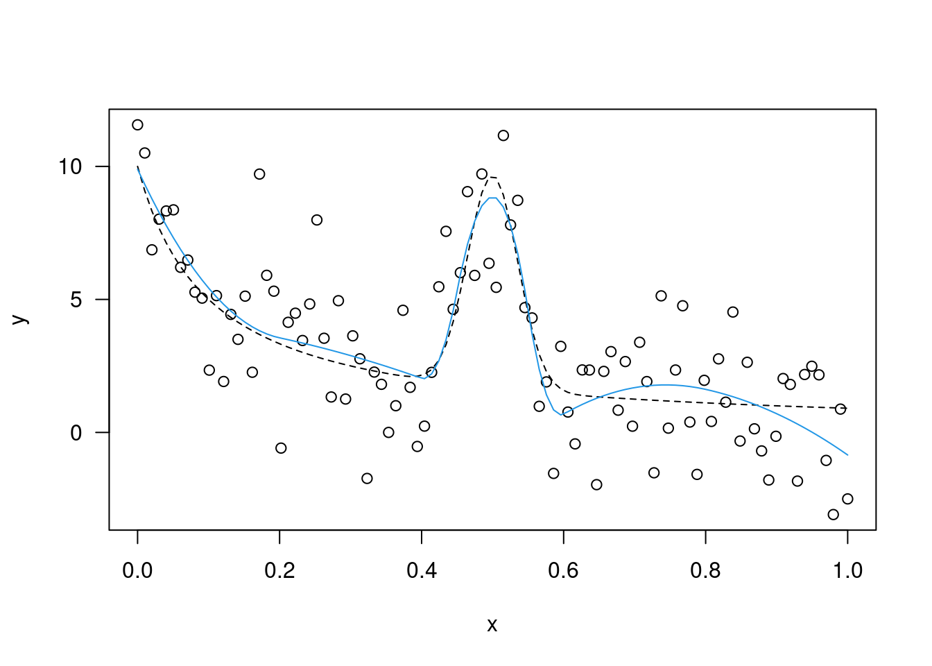
n=30; x=sort(runif(n,0,1)); y=sin(x*pi)+rnorm(n,0,0.1)
plot(x,y); m1=lm(y~x); abline(m1)
x2=x^2; m2=update(m1,~.+x2)
plot(x,y); abline(m1); lines(x,m2$fit,col=2)
##
## Call:
## lm(formula = y ~ x)
##
## Residuals:
##      Min       1Q   Median       3Q      Max
## -0.54263 -0.10194  0.05317  0.19357  0.44373
##
## Coefficients:
##             Estimate Std. Error t value Pr(>|t|)
## (Intercept)   0.8662     0.1116   7.764 1.86e-08 ***
## x            -0.2812     0.1927  -1.459    0.156
## ---
## Signif. codes:  0 '***' 0.001 '**' 0.01 '*' 0.05 '.' 0.1 ' ' 1
##
## Residual standard error: 0.271 on 28 degrees of freedom
## Multiple R-squared:  0.07069,    Adjusted R-squared:  0.0375
## F-statistic:  2.13 on 1 and 28 DF,  p-value: 0.1556
##
## Call:
## lm(formula = y ~ x + x2)
##
## Residuals:
##      Min       1Q   Median       3Q      Max
## -0.14690 -0.05118 -0.02123  0.04942  0.25536
##
## Coefficients:
##             Estimate Std. Error t value Pr(>|t|)
## (Intercept) -0.05135    0.07980  -0.643    0.525
## x            4.12476    0.33616  12.270 1.49e-12 ***
## x2          -4.08321    0.30452 -13.409 1.88e-13 ***
## ---
## Signif. codes:  0 '***' 0.001 '**' 0.01 '*' 0.05 '.' 0.1 ' ' 1
##
## Residual standard error: 0.09973 on 27 degrees of freedom
## Multiple R-squared:  0.8787, Adjusted R-squared:  0.8697
## F-statistic: 97.76 on 2 and 27 DF,  p-value: 4.305e-13
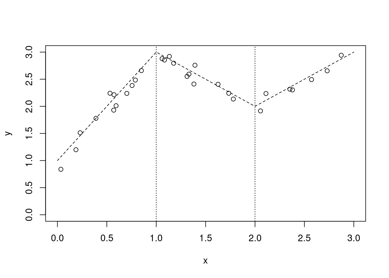
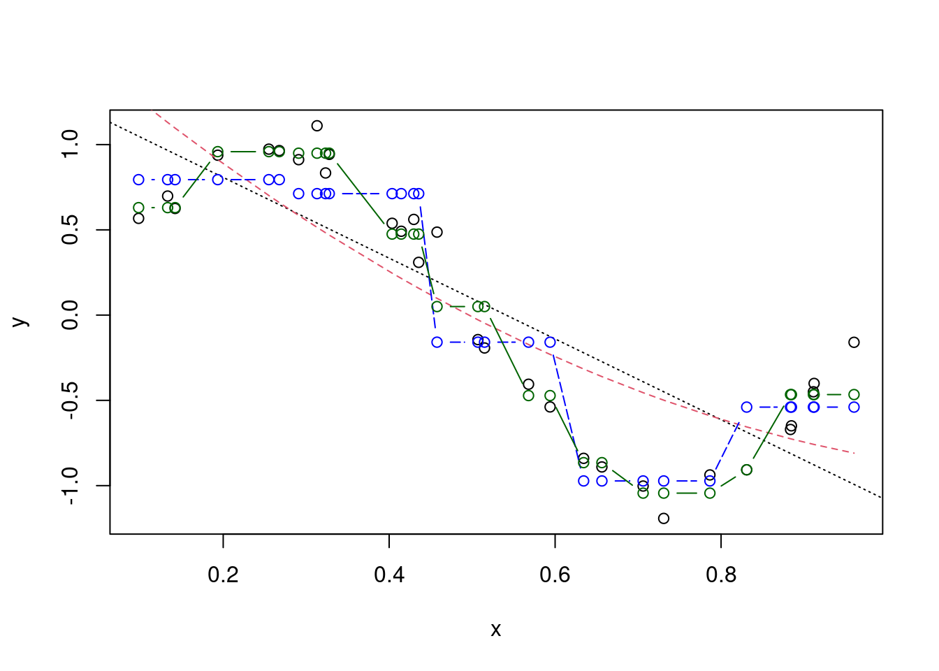
y=sin(x*pi*2)+rnorm(n,0,0.1); plot(x,y); m1=lm(y~x); abline(m1,lty=3)

m2=update(m1,~.+I(x^2));plot(x,y); abline(m1,lty=3);
lines(x,m2$fit,col=2,lty=2)
range(x); cx5=cut(x,5); levels(cx5);
## [1] 0.09806405 0.96024698
## [1] "(0.0972,0.271]" "(0.271,0.443]"  "(0.443,0.615]"  "(0.615,0.788]"
## [5] "(0.788,0.961]"
cx5=cut(x,5,include.lowest=T); levels(cx5)
## [1] "[0.0972,0.271]" "(0.271,0.443]"  "(0.443,0.615]"  "(0.615,0.788]"
## [5] "(0.788,0.961]"
m3=lm(y~cx5);
summary(m3)$coef
##                     Estimate Std. Error     t value     Pr(>|t|)
## (Intercept)       0.79440594  0.1075450   7.3867297 9.744056e-08
## cx5(0.271,0.443] -0.08205625  0.1422687  -0.5767696 5.692526e-01
## cx5(0.443,0.615] -0.95311579  0.1595150  -5.9750845 3.072359e-06
## cx5(0.615,0.788] -1.76686658  0.1595150 -11.0764895 3.918224e-11
## cx5(0.788,0.961] -1.33388708  0.1520916  -8.7702868 4.224418e-09
## [0.0972,0.271]  (0.271,0.443]  (0.443,0.615]  (0.615,0.788]  (0.788,0.961]
##      0.7944059      0.7123497     -0.1587098     -0.9724606     -0.5394811
plot(x,y); abline(m1,lty=3); lines(x,m2$fit,col=2,lty=2)
lines(x,m3$fit,col="blue",lty=5,type="b")
cx10=cut(x,10,include.lowest=T); m4=update(m3,~cx10)
plot(x,y); abline(m1,lty=3); lines(x,m2$fit,col=2,lty=2)
lines(x,m3$fit,col="blue",lty=5,type="b");
lines(x,m4$fit,col="darkgreen",lty=1,type="b")
Local polynomial estimator
est=locpoly(xis, bandwidth = 0.25); do=density(xis);
hist(xis,prob=T,ylim=c(0,0.6),xlim=range(est$x,xis,do$x),las=1)
lines(est$x,est$y); lines(do$x,do$y,col=2)
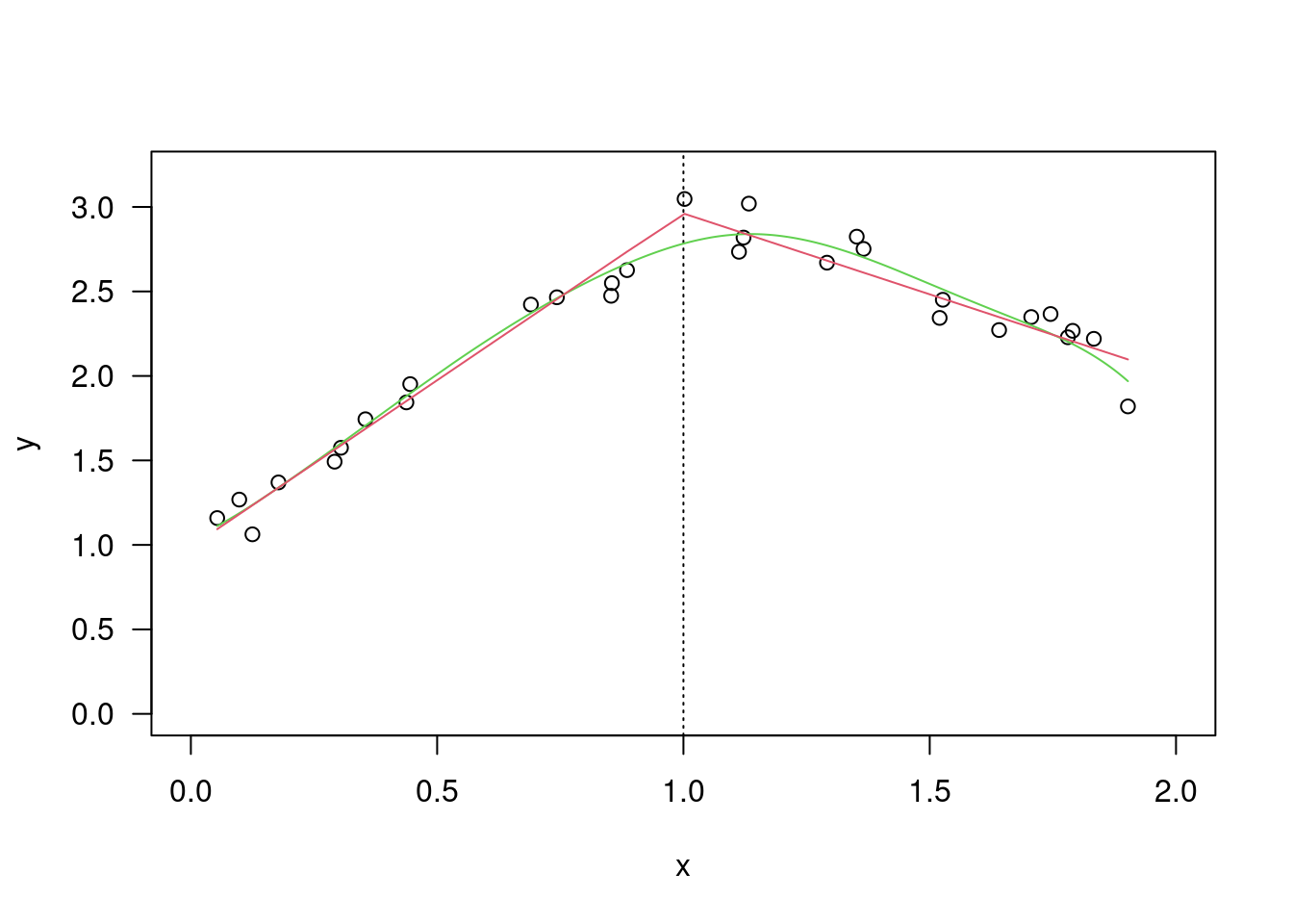
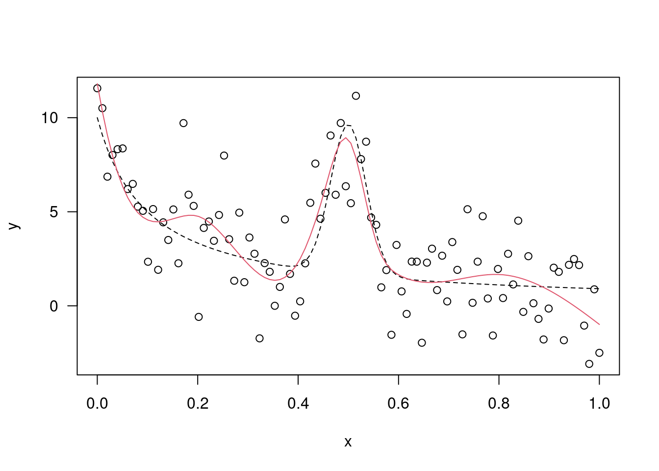
plot(xis, yis,xlab="Duration",ylab="Waiting",las=1)
fit1=locpoly(xis, yis, degree=1,band= 0.25); lines(fit1,col=2)
fit2=locpoly(xis, yis, degree=2,band= 0.25);lines(fit2,col=4)
fit3=locpoly(xis, yis, degree=2,band= 0.5);lines(fit3,col=3)